User guide
TissueMAPS uses the client-server model, where clients can make requests to the server via a REST API using the Hypertext Transfer Protocol (HTTP).
Most users will interact with the server via the browser-based interface. However, additional HTTP client implementations are provided via the tmclient package, which allows users to interact more programmatically with the server. These use cases are covered in the section interacting with the server.
The server handles client requests, but delegates the actual processing to the tmlibrary package. The TissueMAPS library provides active programming (API) and command line interfaces (CLI), which can also be used directly, i.e. in a server-independent way. This is covered in the section using the library.
Interacting with the server
This section demonstrates different ways of interacting with a TissueMAPS server. All of them of course require access to a running server instance. This may either be a production server that you access via the internet or a development server running on your local machine. The following examples are given for localhost, but they similarly apply a server running on a remote host.
Tip
Here, we connect to the server using URL http://localhost:8002. The actual IP address of localhost is 127.0.0.1 (by convention). It’s possible to use the name localhost, because this host is specified in /etc/hosts. So when you are running the TissueMAPS server on a remote host in the cloud instead of your local machine, you can use the same trick and assign a hostname to the public IP address of that virtual machine. To this end, add a line to /etc/hosts, e.g. 130.211.160.207 tmaps. You will then be able to connect to the server via http://tmaps. This can be convenient, because you don’t have to remember the exact IP address (which may also be subject to change in case you don’t use a static IP address). Note that you don’t need to provide the port for the production server, because it will listen to port 80 by default (unlike the development server, who listens to port 8002).
User interface
Enter the IP address (and optionally the port number) of the server in your browser. This directs you to the index site and you are asked for your login credentials.

Login prompt.
User panel
After successful authorization, you will see an overview of your existing experiments.
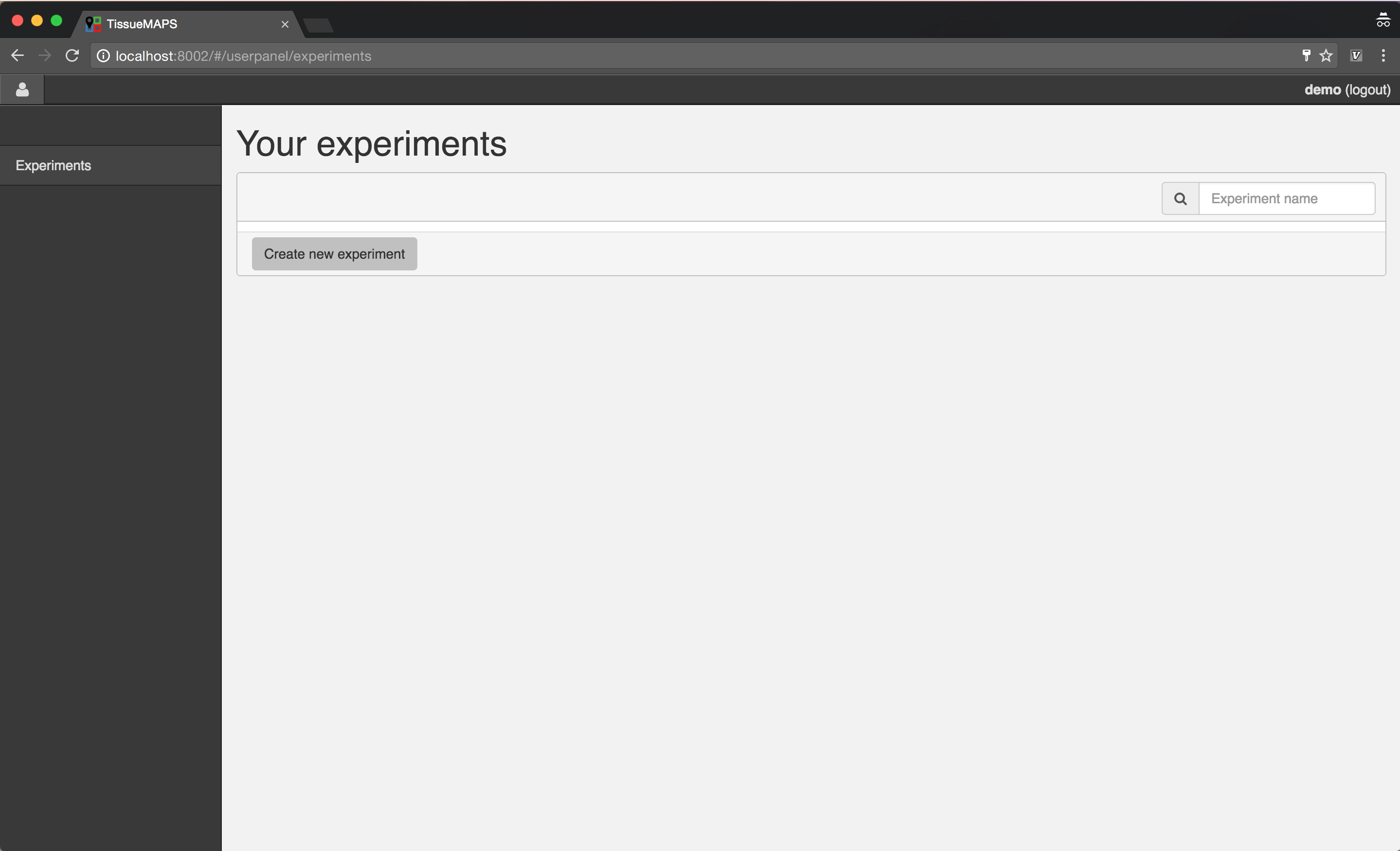
Experiment overview.
Creating an experiment
To create a new experiment, click on  .
.

Experiment creation.
When you click on  , the experiment gets created and you get directed back to the overview.

Experiment overview.
Note
By default, experiments can only be viewed and modified by the user who created them, but they can be shared with other users. However, this functionality is currently only available via the API (see ExperimentShare).
Next, you can upload images and process them. To this end, click on  , which directs you to the workflow manager.
Workflow manager
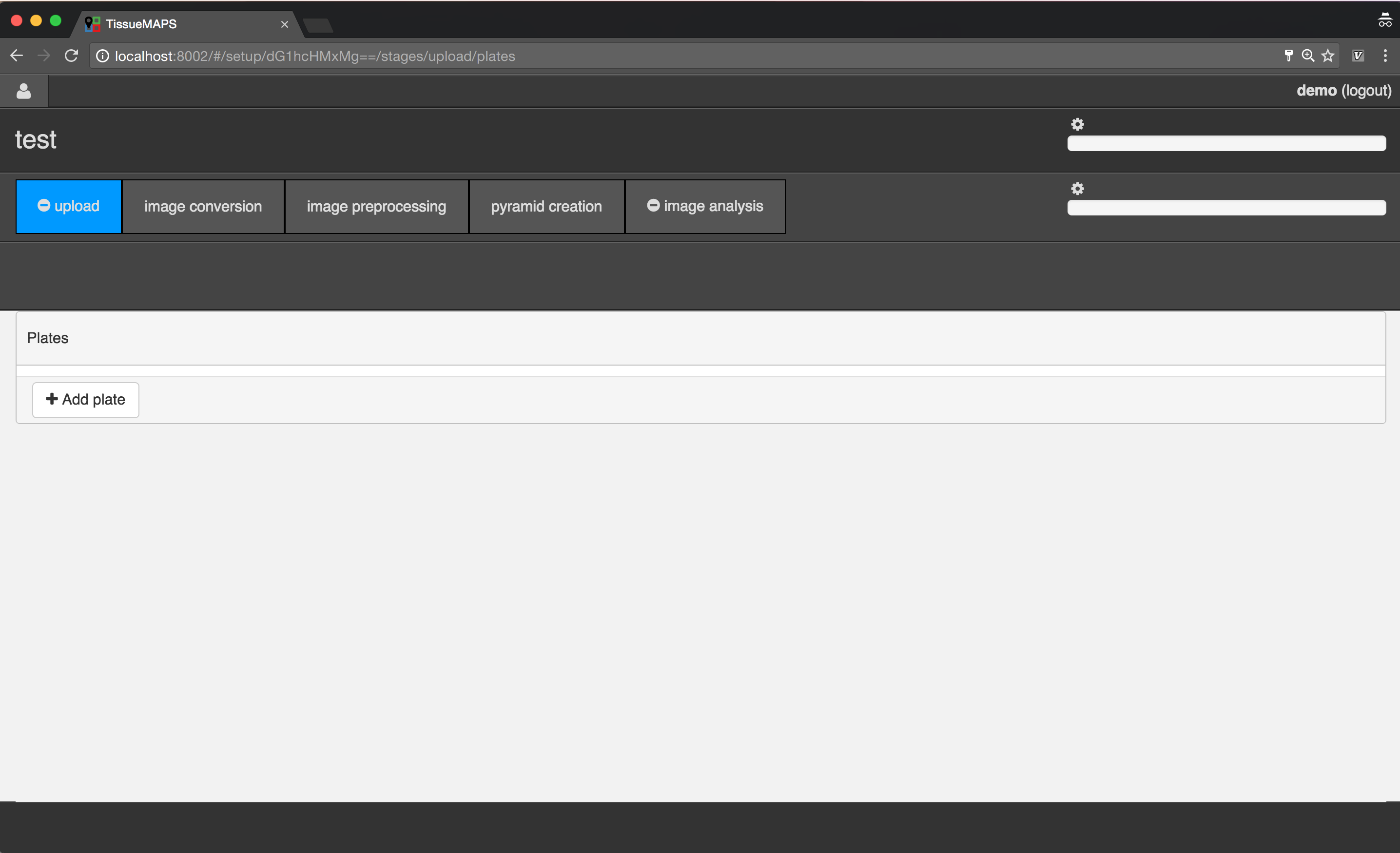
Workflow manager.
Uploading image files
To begin with, add a new plate, by clicking on  .
.

Plate creation.
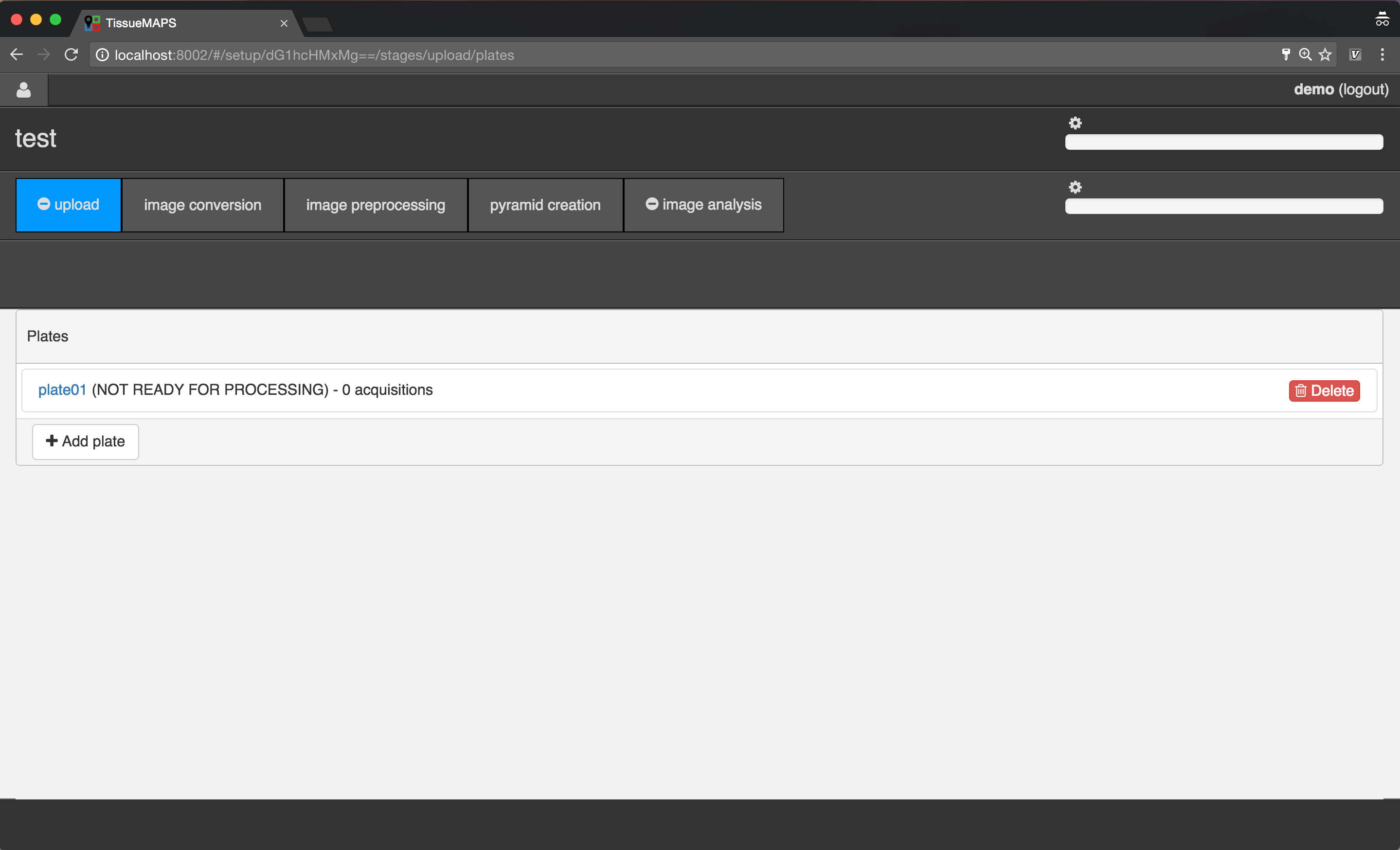
Plate overview.
Select the created plate, by clicking on the link  .
.
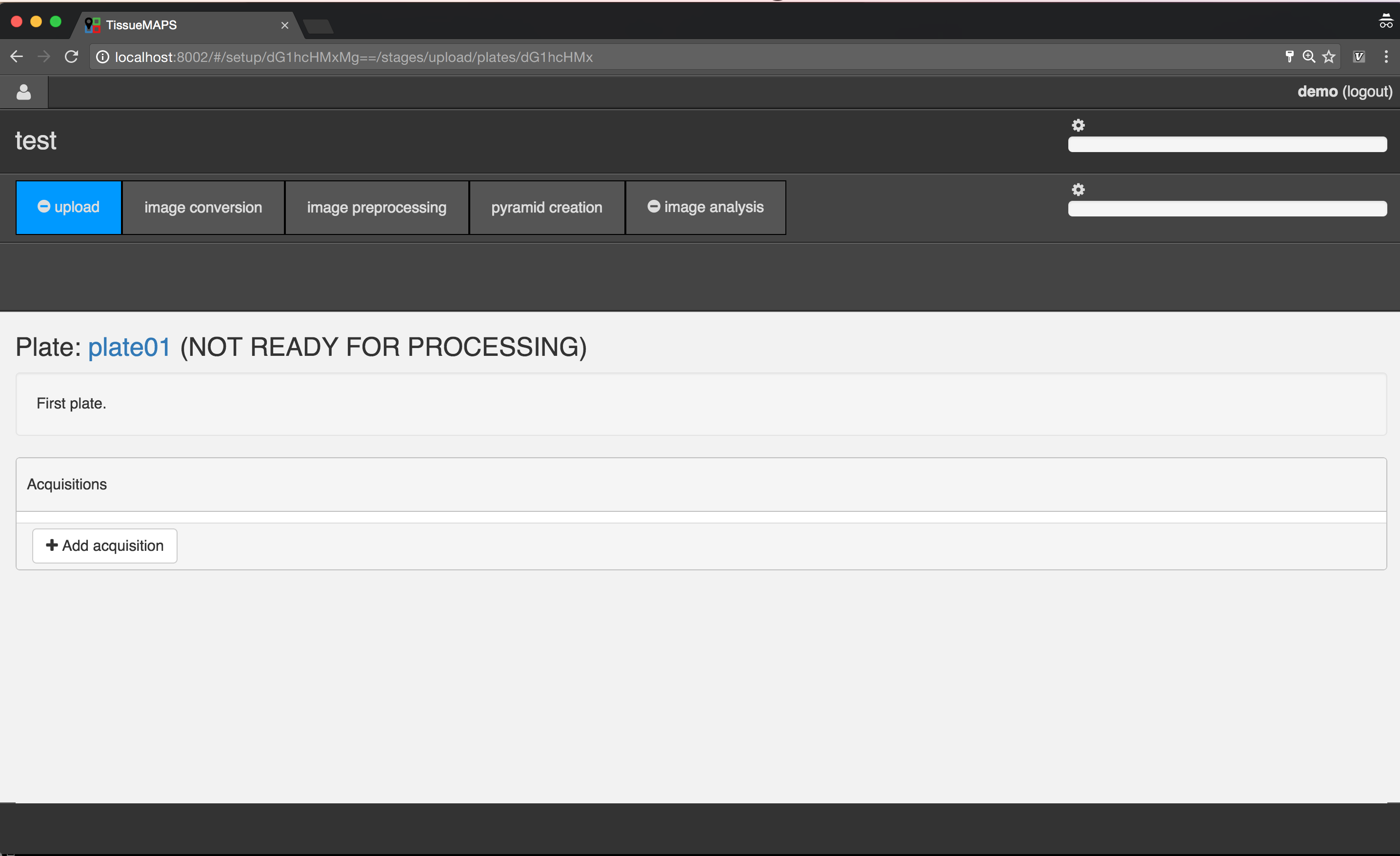
Acquisition overview.
Add a new acquisition, by clicking on  .
.

Acquisition creation.
Acquisition overview.
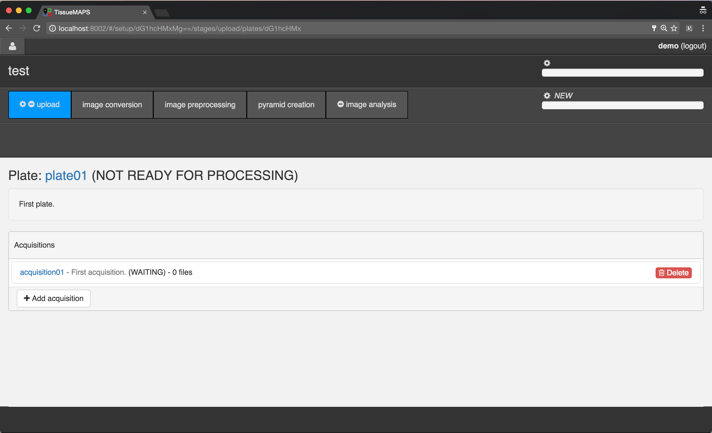
Select the created acquisition, by clicking on the link  .
.
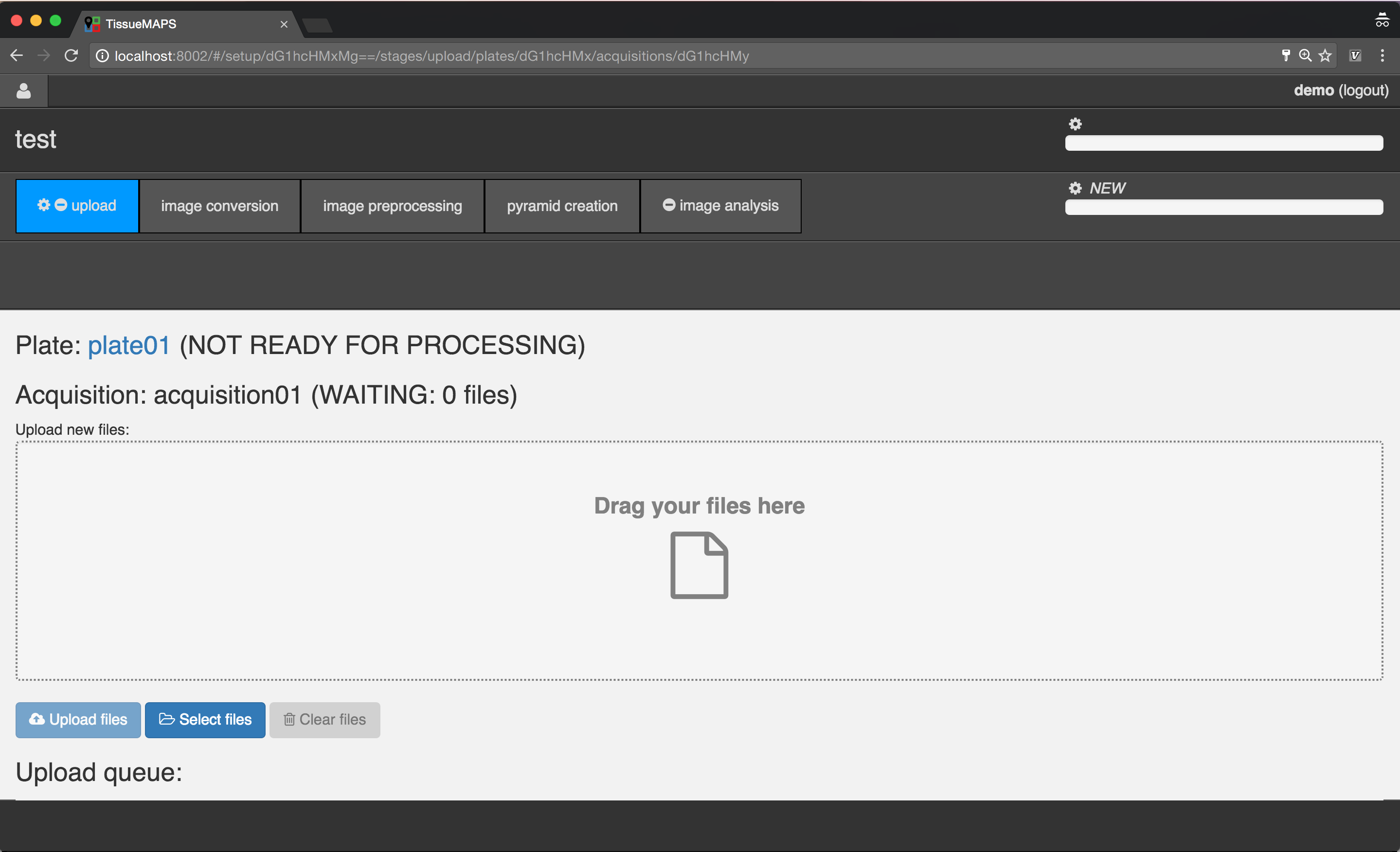
Upload.
 . Then click on
  to start the upload process.
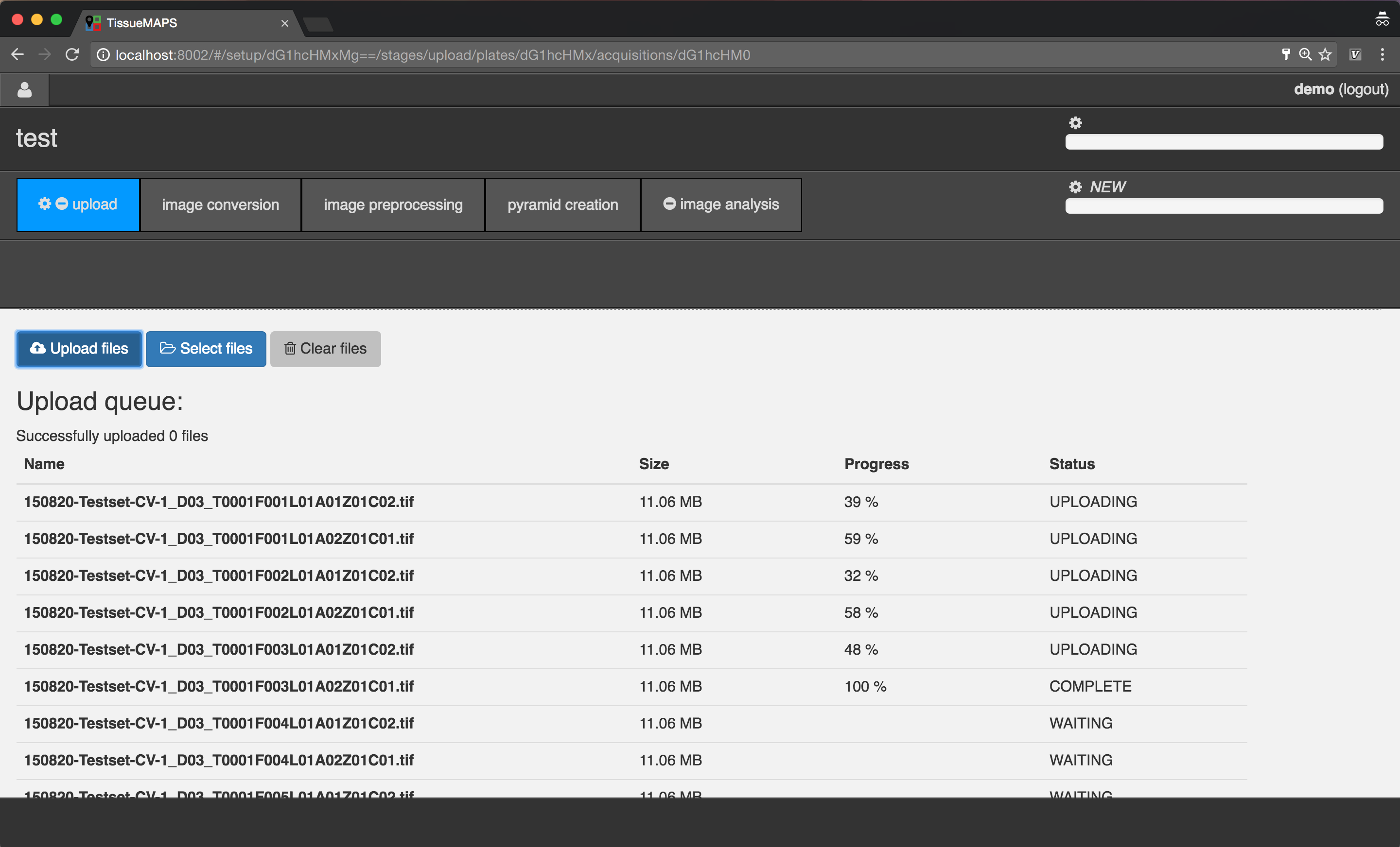
Upload in process.
Note
File upload via the user interface works reliable for serveral thousand images. When uploading tens or hundreds of thousands of images, we recomment uploading files via the command line instead. To this end, you can use the tm_client tool provided by the tmclient package.
Note
The upload process will be interrupted when the page is reloaded. However, you can simply add the files afterwards again and restart uploading. The server keeps track of which files have already been uploaded and won’t upload them again.

Plate overview.
You can add additional acquisitions and plates to the experiments by repeating the steps described above. Once you have uploaded all files, you can continue to process them.
Processing images
Once you have uploaded all files, you can proceed to the subsequent processing stages.
Note
You are prevented from proceeding until upload is complete. Requesting this information from the server may take a few seconds for large experiments.
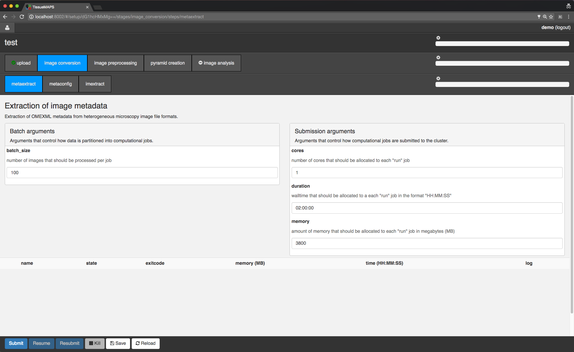
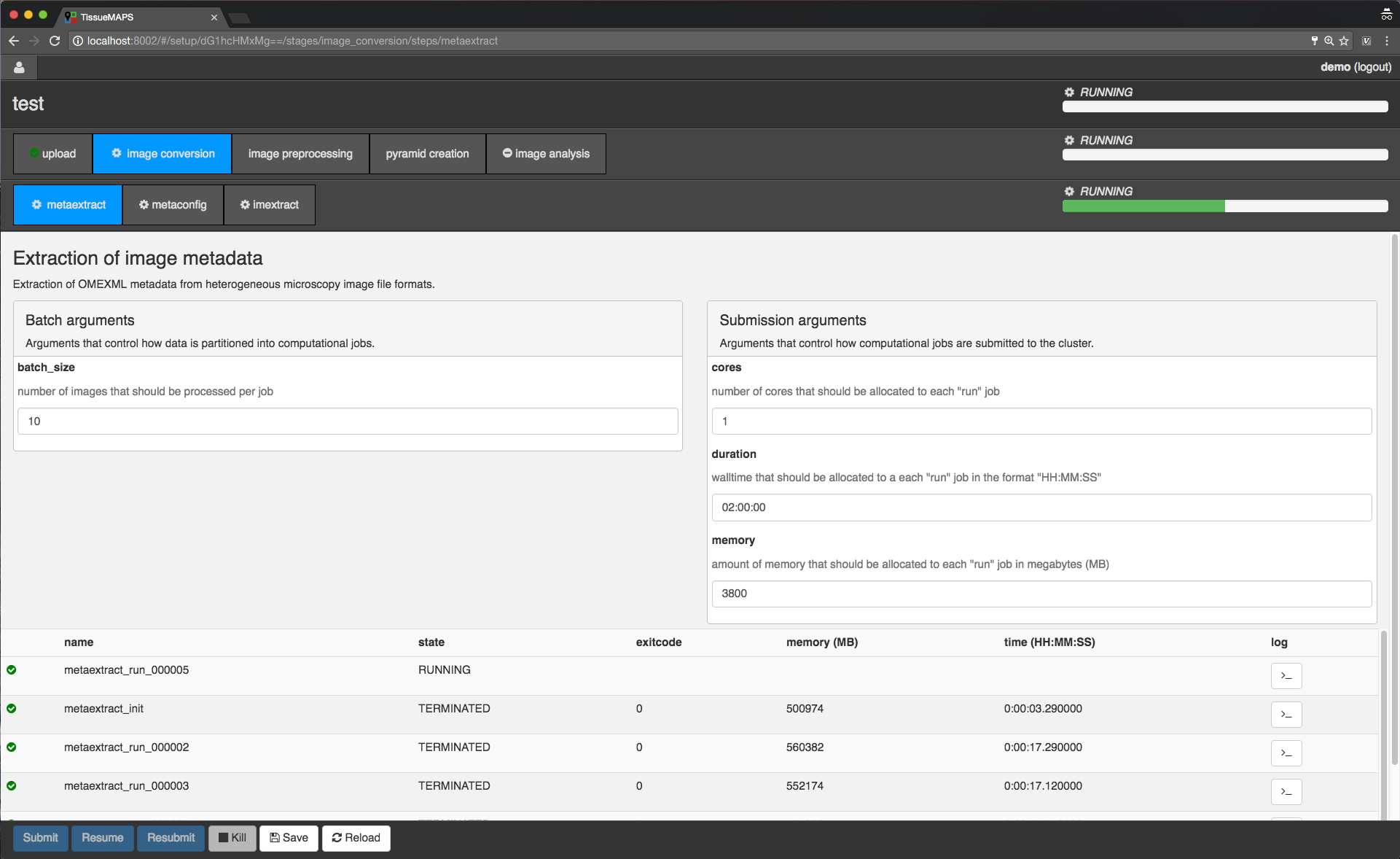
Workflow control panel.
You can toggle between different stages and steps. The view applies to the currently active combination of stage and step - in this case “image convesion” and “metaextract”, respectively.
The loading bars indicate the progress of workflow, stage and step. They are green by default, but turn red as soon as a single job failed. Above the loading bars, you can see the current processing state (e.g. “SUBMITTED”, “RUNNING”, or “TERMINATED”). When the currently active stage or step is in state “RUNNING”, the cog wheel above the loading bar will also start spinning. The cog will also appear on the stage and step tabs to indicate the state of stages or steps, which are not selected at the moment.
In the main window you can set “batch” and “submission” arguments to control the partition of the computational task into individual jobs and the allocation of resources for each job, respectively. Upon submission, individual jobs will be listed below the argument section. If required arguments are missing for a stage or step, this will be indicated on the corresponding tab by a minus (visible for the “image analysis” stage). In this case, you cannot submit these stages without providing the missing arguments.
Since the workflow hasn’t been submitted yet, the loading bars are all set to zero and no jobs are listed.
You can click through all stages and steps and set arguments according to your needs. Once you are happy with your settings, you can either  the settings or
  the workflow for processing (settings get also automatically saved upon submission).
Note
Submission depends on the current view. Only the currently active stage as well as stages to the left will be processed. For example, if you are in stage “image preprocessing” and you click on , only stages “image conversion”, “image preprocessing” and “pyramid creation” will be submitted.
Note
Arguments batch_size and duration depend on each other. The larger the batch, i.e. the more images are processed per compute unit, the longer the job will typically take.
Note
Arguements cores and memory depend upon the available compute resources, i.e. the number of CPU cores and the amount of RAM available per core. The defauls of 3800MB applies to the default machine type flavor at ScienceCloud at University of Zurich and may need to be adapted for other clouds.
For now, let’s submit the workflow from the first stage “image conversion”.
Workflow submission in progress.
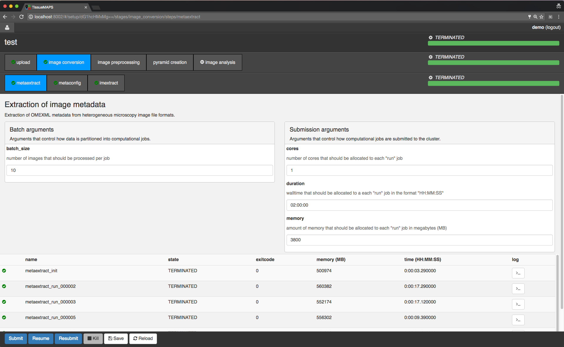
Workflow submission done.
Note
Once a workflow has been submitted, you can safely close the window or disconnect from the internet, since the jobs are processed remotely on the server in an asynchronous manner.
Once stage “image conversion” is done, you can proceed to any other stage and click on  . Alternatively, you could have submitted a further downstream stage in the first place.
For the purpose of this demo, we will proceed to stage “pyramid creation” and resume the workflow.
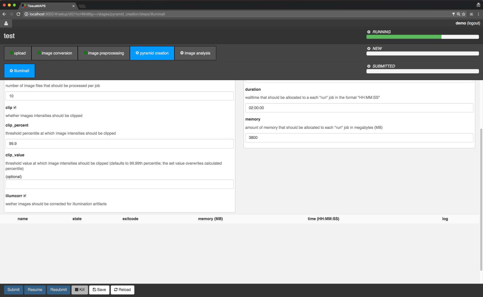
Workflow submission resumed.
Note
Once stage “pyramid creation” is done, you can already view the experiment. However, you won’t be able to visualize segmented objects on the map. To this end, you first need to process stage “image analysis”.
You can further  the workflow with modified arguments from any stage afterwards.
The image analysis stage is a bit more complex, therefore we will cover it in a separate section.
Setting up image analysis pipelines
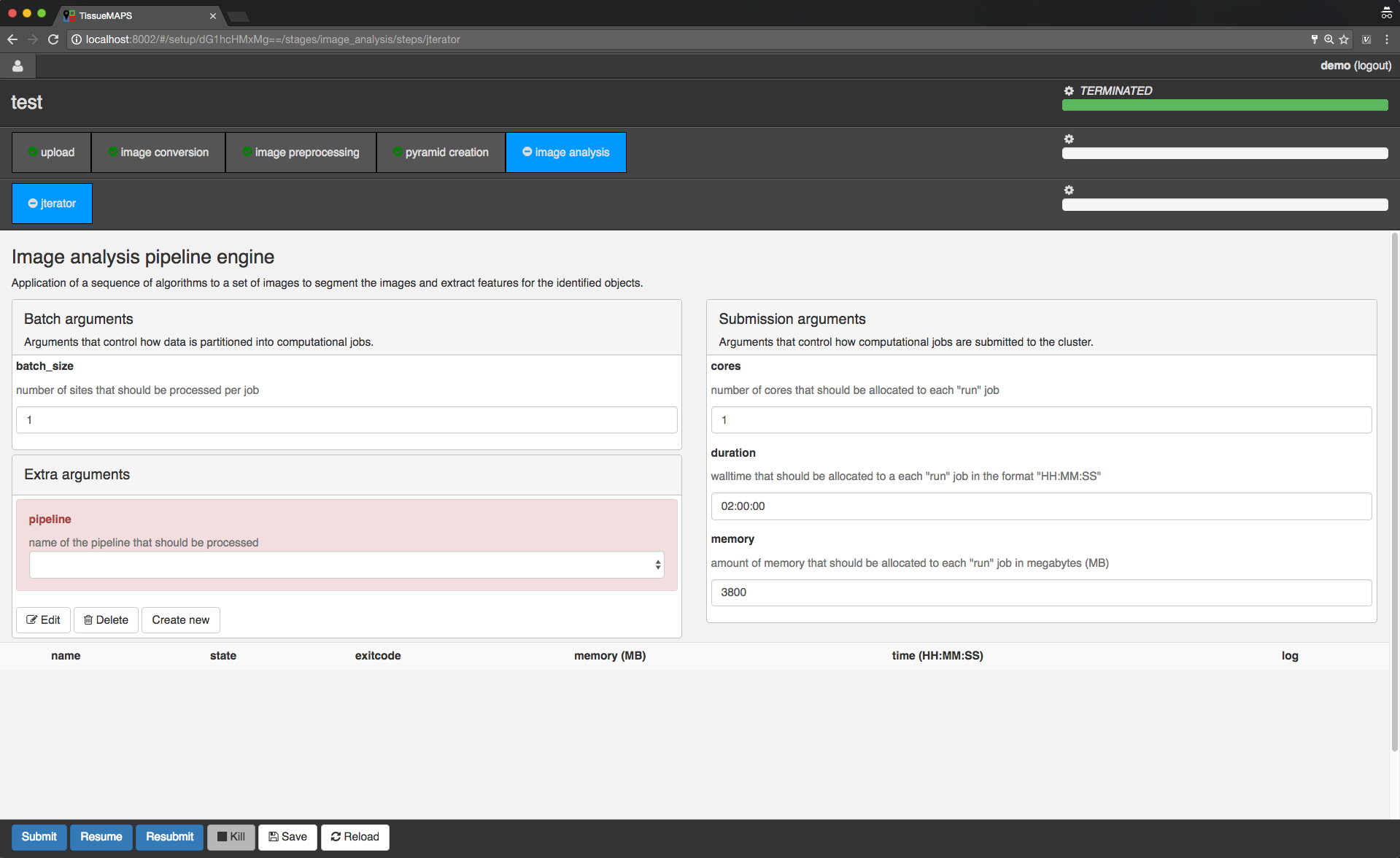
Image analysis stage.
To begin with, you need to create a pipeline. To this end, click on  . Give the pipeline a descriptive name, here we call it
 test-pipe.
This will direct you to a separate interface for defining the pipeline.
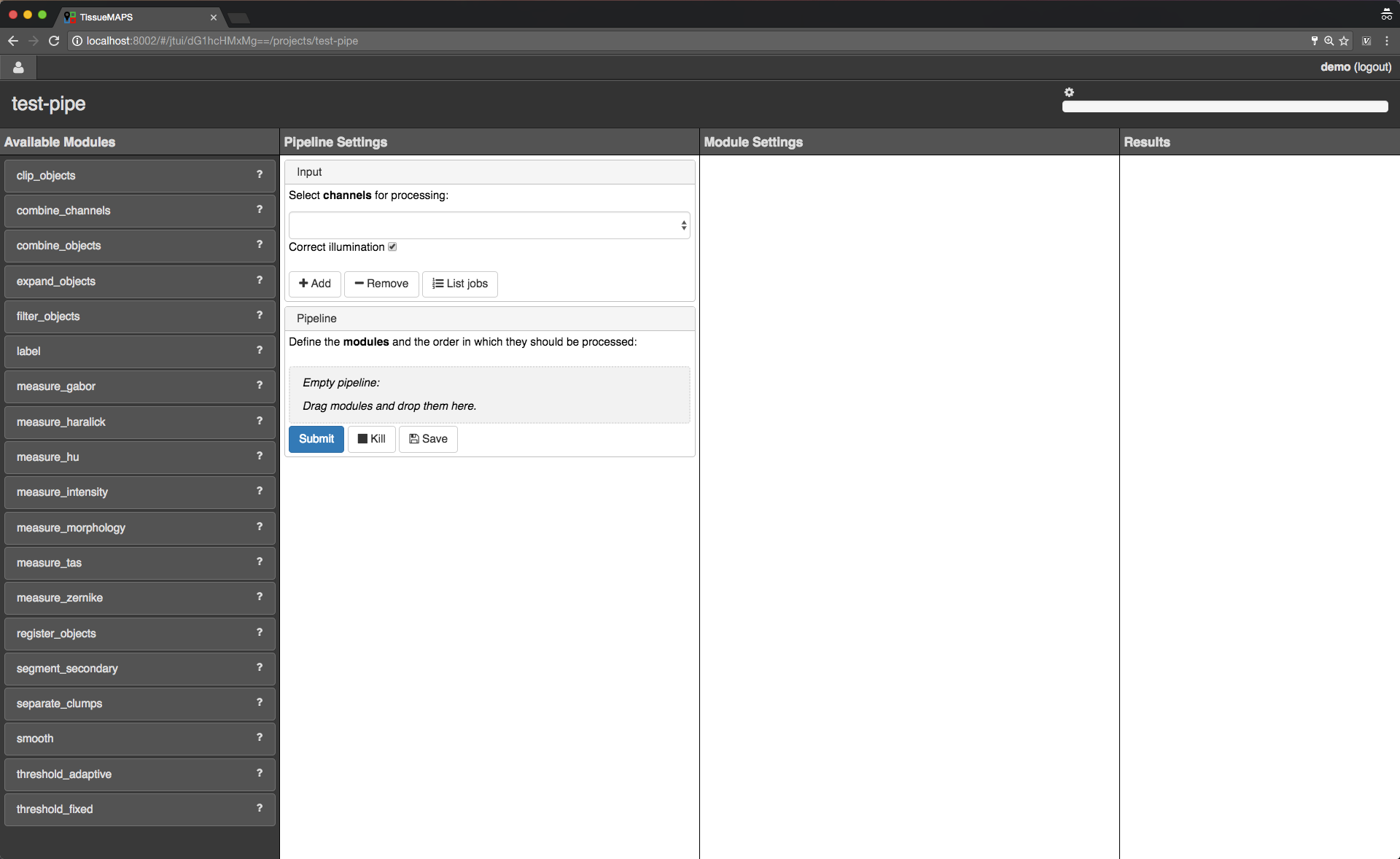
Jterator interface.
jtmodules package. “Pipeline Settings” describes the input for the pipeline in form of “channels” and lists modules that have been added to the pipeline. The module “Module Settings” section describes input arguments and expected outputs of the currently selected module.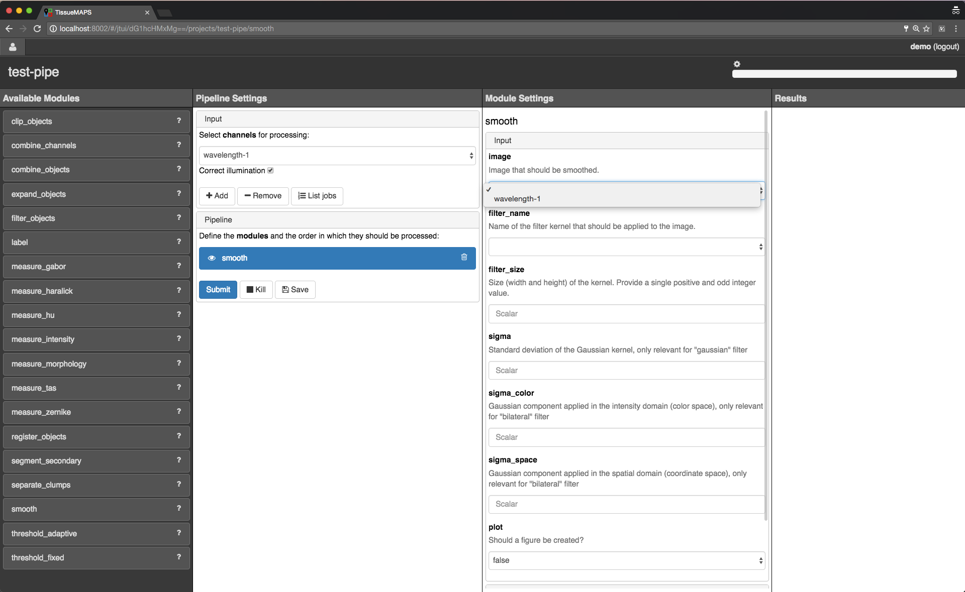
Pipeline and module settings.
You can drag and drop modules from the list of available modules into the indicated field in the pipeline section and then click on added item to set module parameters. The order of modules in the pipeline can be rearranged by dragging them up or down.
You can further select channels in the input section to make them available to the pipeline. Additional channels can be removed when neeeded. The selected “channels” become available as an input for the selected module.
Tip
Images for all channels selected in the input section will be loaded into memory (for the acquisition site corresponding to the given batch). So remove any channel you don’t use in your pipeline to gain performance.
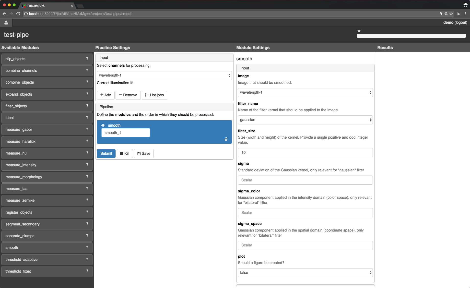
Module renaming.
Note
Names of modules in the pipeline must be unique. When adding the same module twice, it will be automatically renamed by appending it with a number. Be aware that names of module outputs must be hashable and therefore also unique. Best practice is to use to use the module as a namespace: <module_name>.<output_argument_name>, e.g. smooth.smoothed_image for the above example. Since module names must be unique the resulting output will consequently have a unique name, too.
Add all modules to the pipeline that you need for your analysis and set parameters.
Note
Types of input parameters are checked internally. Only inputs matching the type definition of the input argument are listed in the drop-down menue.
Here, we will first add all the modules required to segment “Nuclei” and “Cells” in the images.
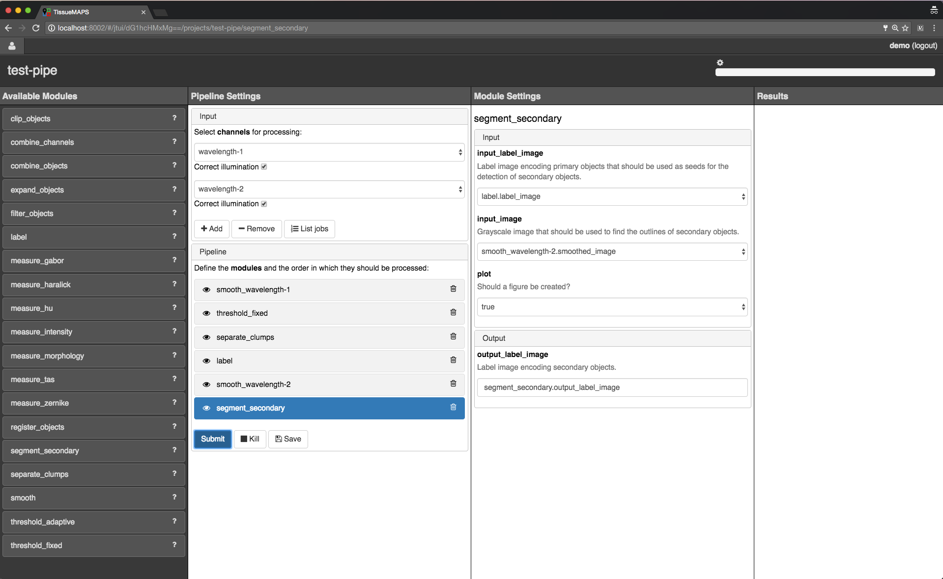
Example segmentation pipeline.
The pipeline can be saved at any time by clicking on . This will save the pipeline settings as well as settings of each module in the pipeline.
When all required parameters are set, the pipeline can be submitted by clicking on (submission will automatically save the pipeline as well).

Pipeline submission.
To see which acquisition sites the jobs map to, click on  .
.
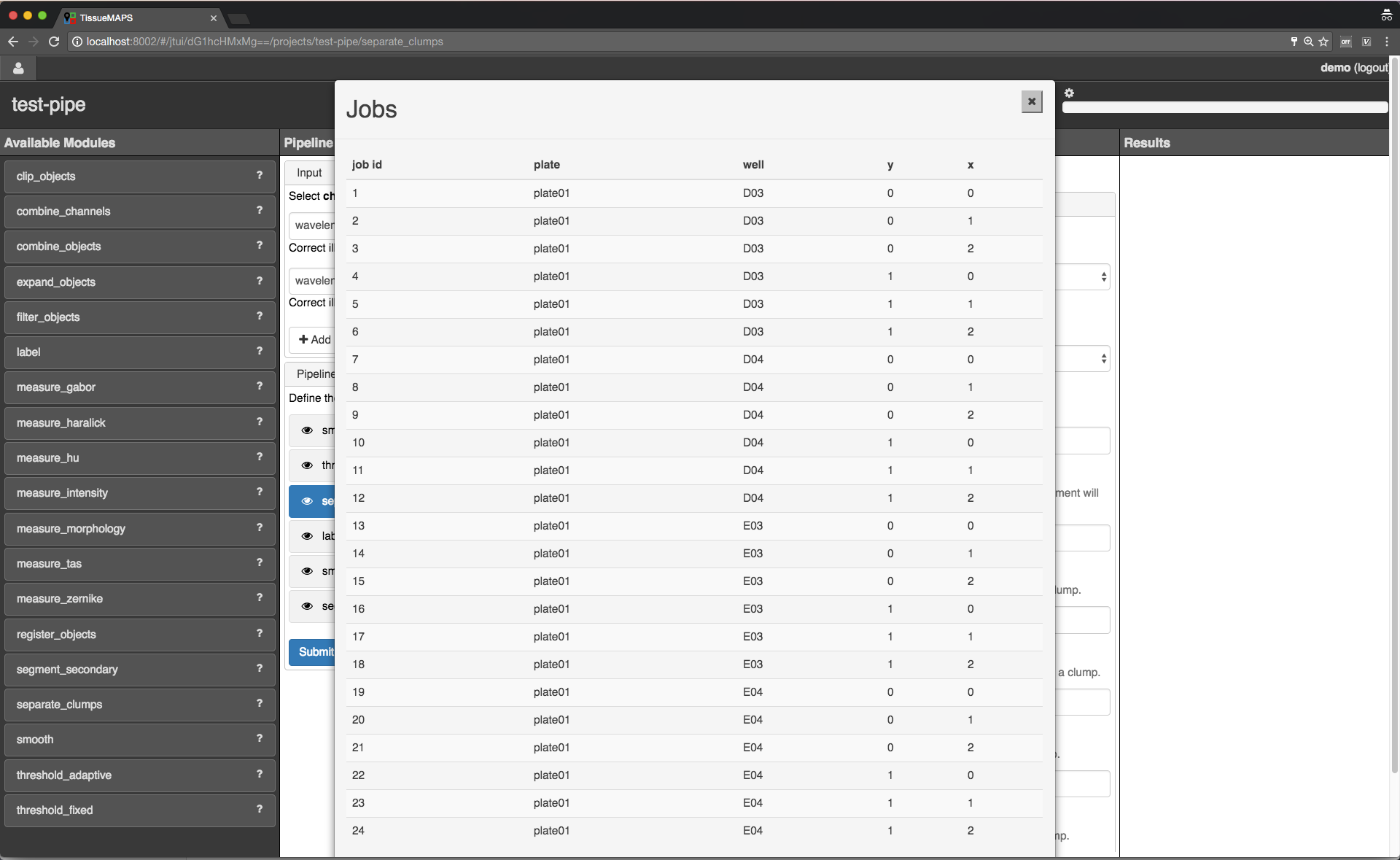
Job list.
site corresponding to a particular job. This is intended to help you select job IDs for testing your pipeline, such that you include images from different wells or positions within a well.Note
In the workflow panel you can set a batch_size for the “jterator” step. However, when you submit the pipeline for testing in the jterator user interface, batch_size will be automatically set to 1, such that only one acquisition site will be processed per job.
Once submitted, jobs get cued and processed depending on available computational resources. If you have access to enough compute units, all jobs will be processed in parallel.
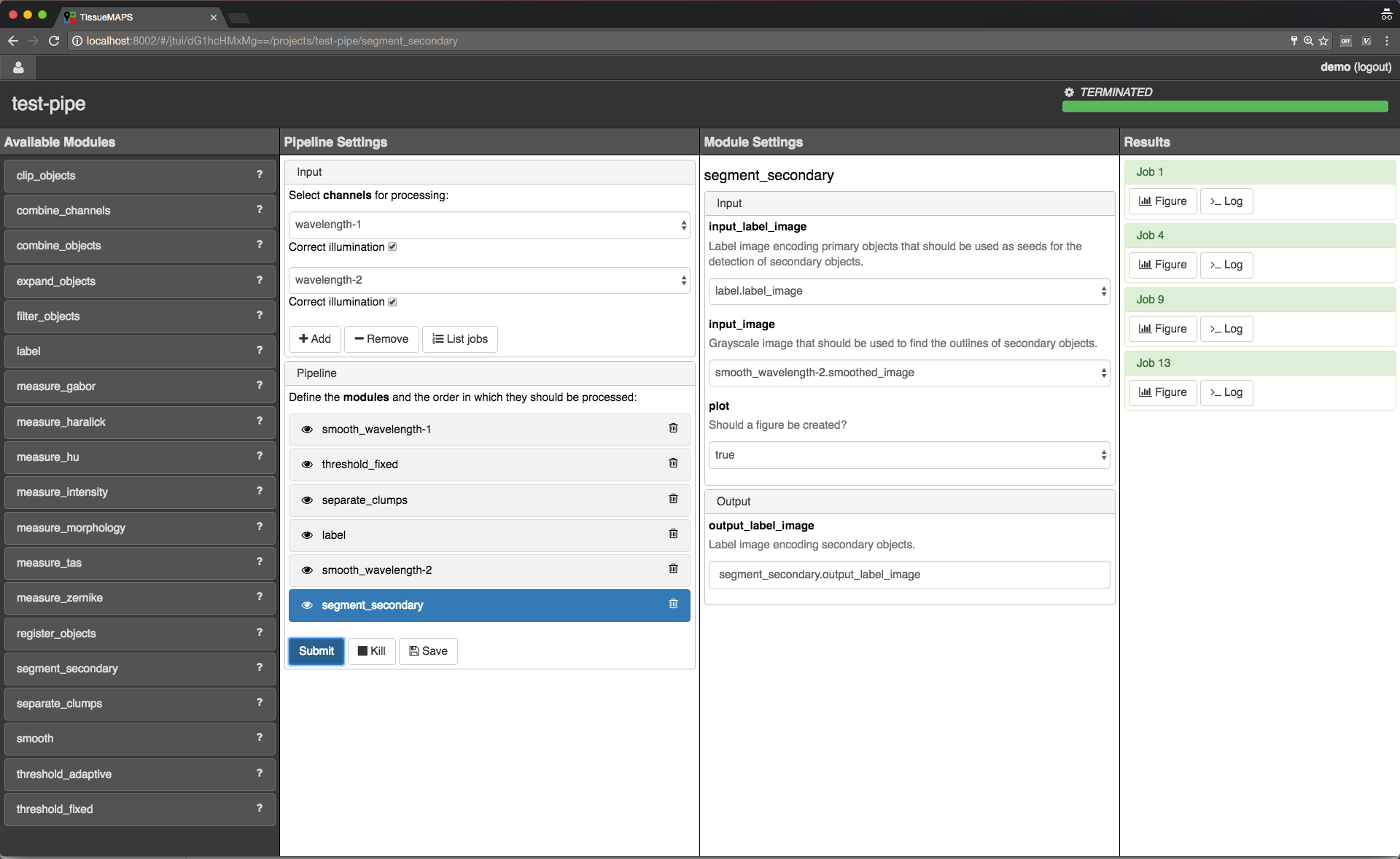
Pipeline results.
 is active for the currently selected module.
When clicking on , the figure for the respective job is displayed in fullscreen mode.
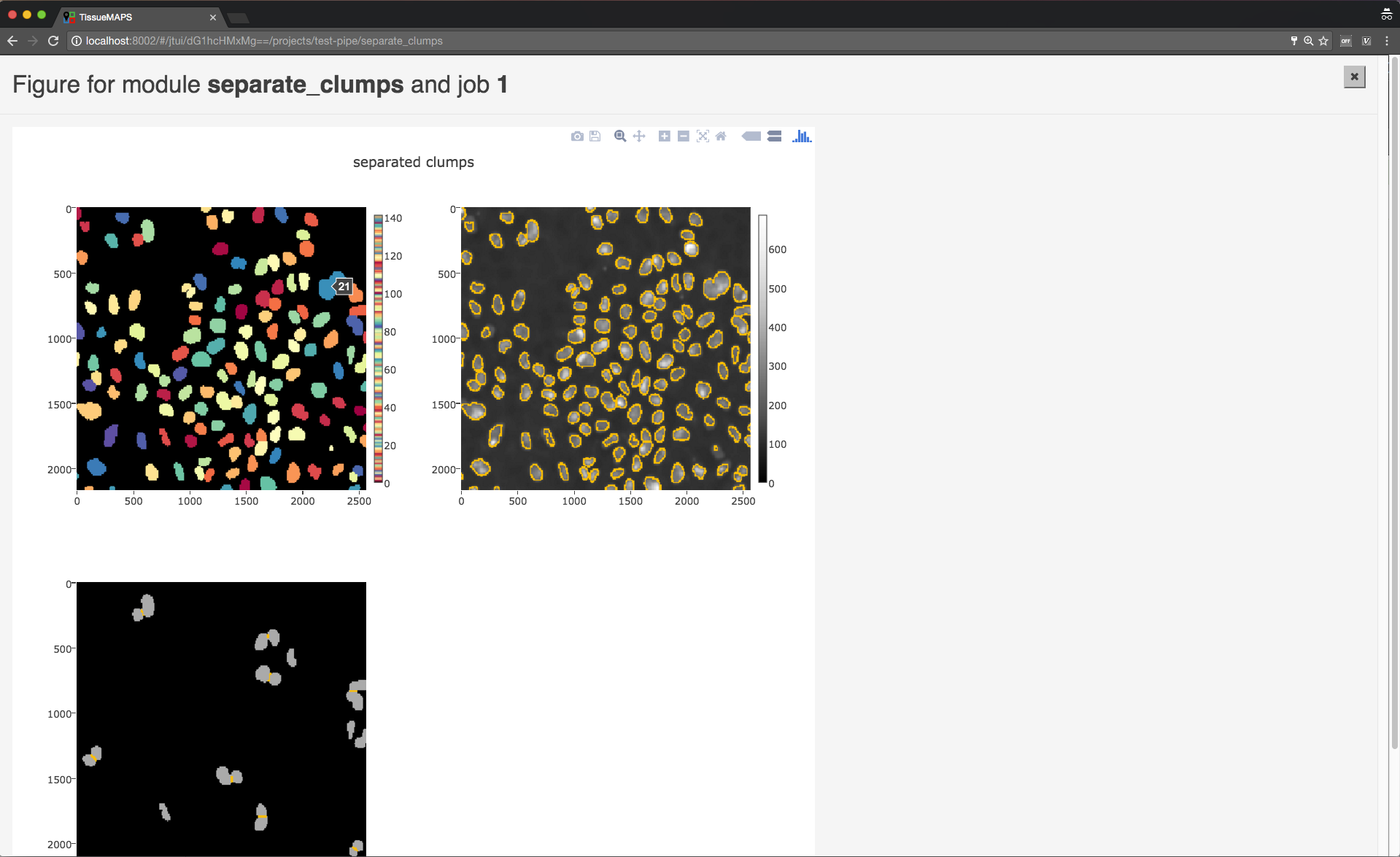
Module figures.
Note
Plotting needs to be explicitely activated for a module by selecting true for argument “plot”. This is done to speed up processing of the pipeline.
When clicking on  , the log output for the respective job is displayed. The messages includes the log of the entire pipeline and is the same irrespective of which module is currently active.
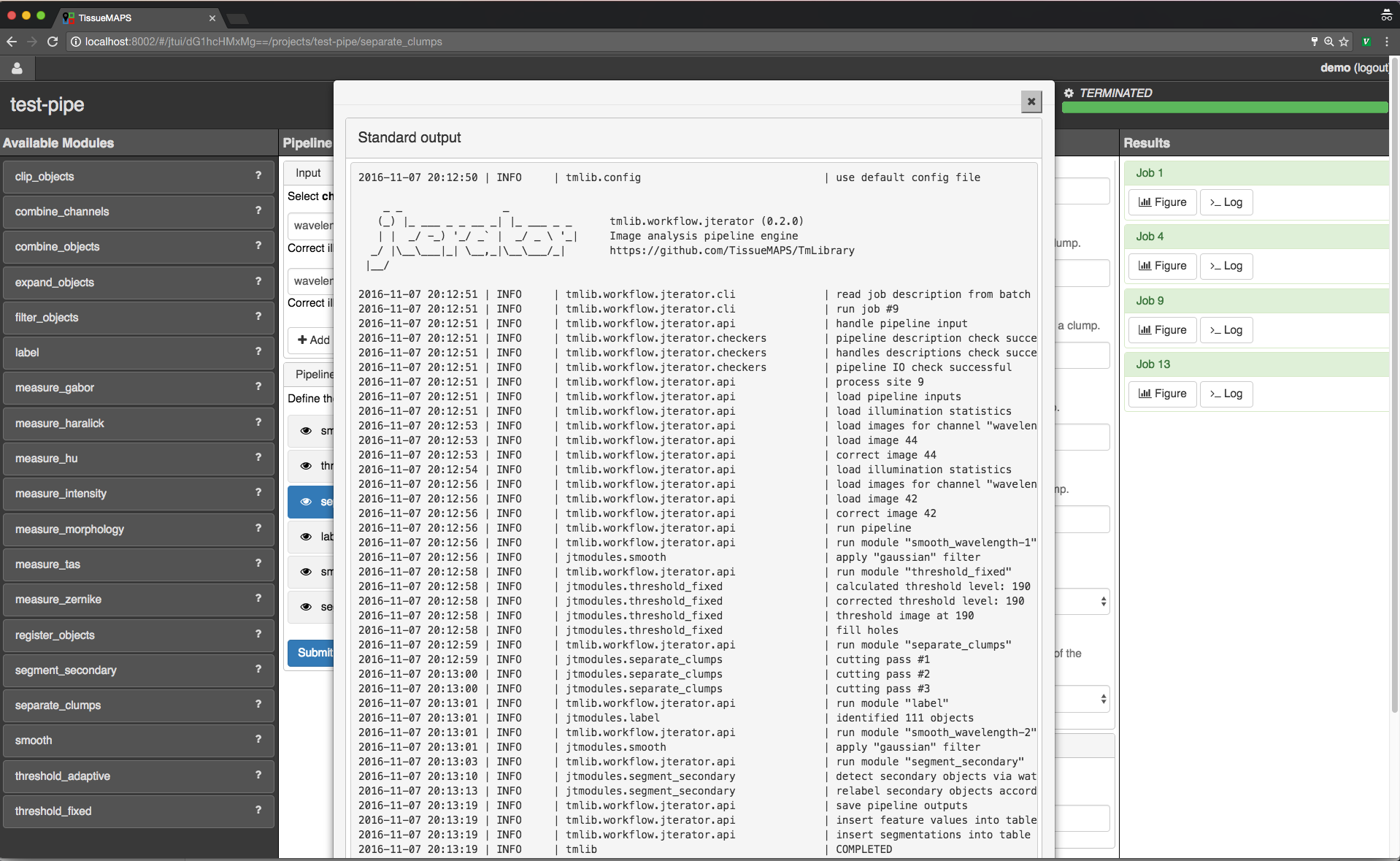
Pipeline log outputs.
INFO by default.To save segmented objects and be able to assign values of extracted features to them, objects need to be registered using the register_objects modules. From a user perspective, the registration simply assigns a name to a label image.
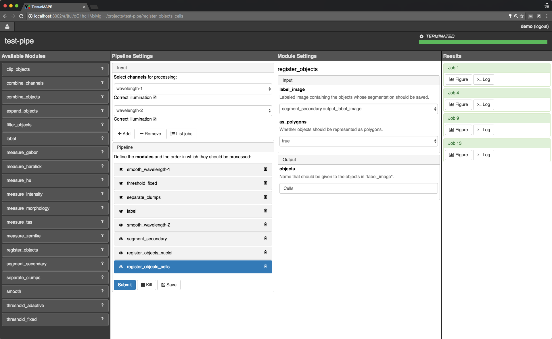
Object registration.
label module, for example.When we are happy with the segmentation results, we can add addtional modules for feature extraction.
Warning
All extracted features will be automatically saved. Since the resulting I/O will increase processing time, its recommended to exclude measurement modules from the pipeline for tuning segmentation parameters.
Tip
You can inactivate modules by clicking on  without having to remove them from the pipeline. Just be aware that this may affect downstream modules, since the output of inactivated modules will of course no longer be produced.
Tip
You can quickly move down and up in the pipeline in a Vim-like manner using the j and k keys, respectively.
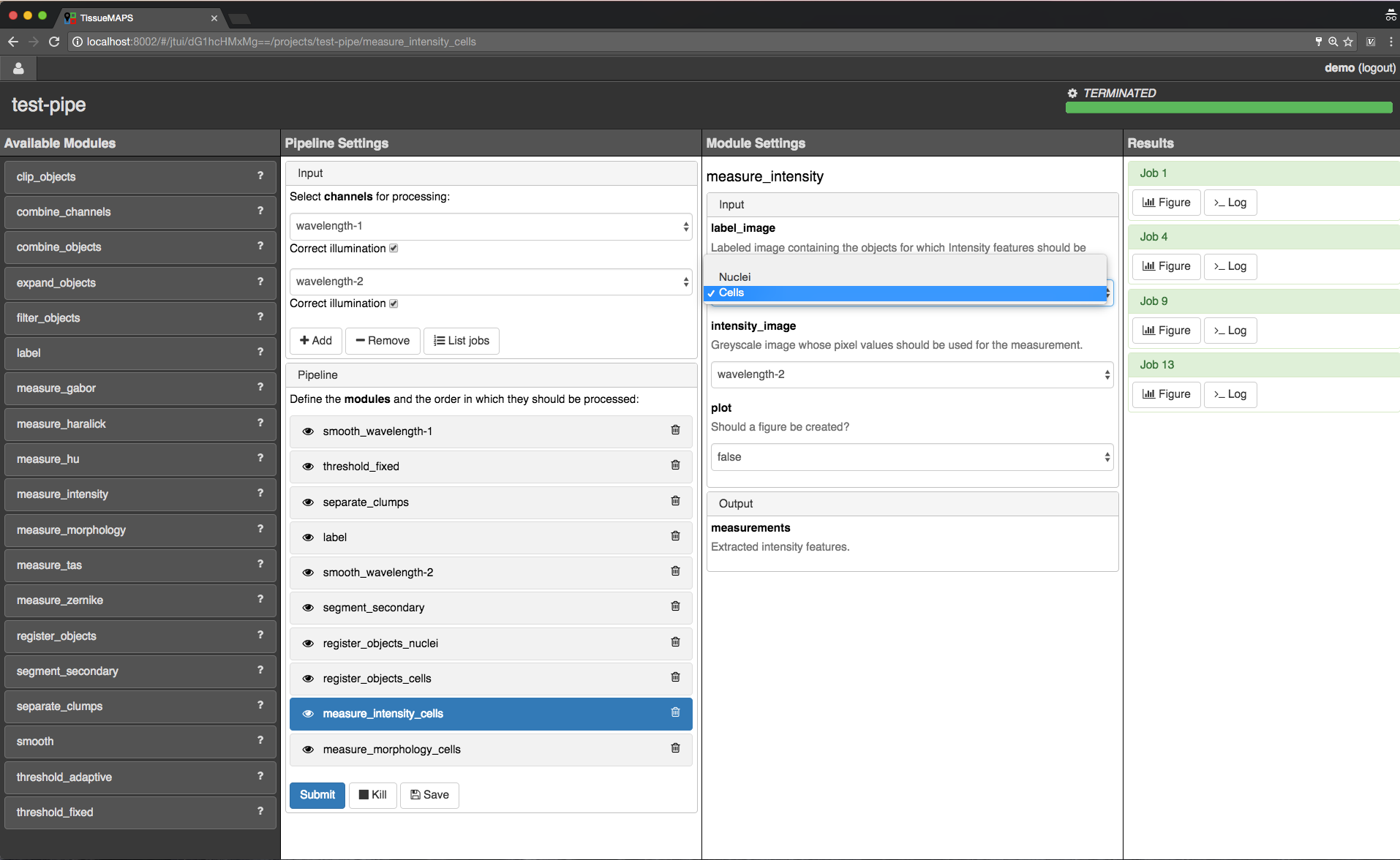
Feature extraction.
intensity require an additional raster image. Others, such as morphology measure only object size and shape and are thus independent of the actual pixel intensity values.Note
Feature names follow a convention: <class>_<statistic>_<channel>. In case features are intensity-independent, the name reduces to <class>_<statistic>. For the above example this would result in Intensity_mean_wavelength-2 or Morphology_area.
Once you have set up your pipeline, save your pipeline (!) and return to the workflow panel. Select the created pipeline and submit the “image analysis” stage by clicking on . In contrast to submissions in the jterator user interface, this will now submit all jobs and potentially run more than one pipeline per job in a sequential manner, depending on the specified batch_size.
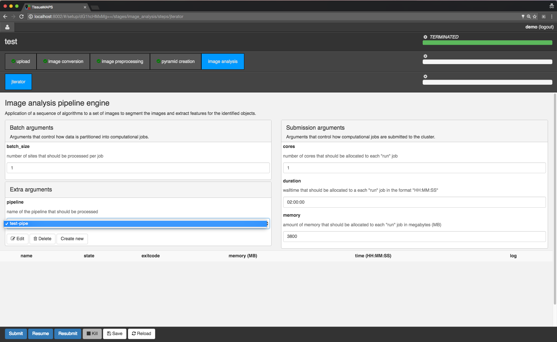
Image analysis submission.
 the workflow settings.
Viewer
Once you’ve setup your experiment, you can view it by returning to the user panel and clicking on  .
.
The MAP
The interactive MAP is the centerpiece of TissueMAPS (as the name implies).
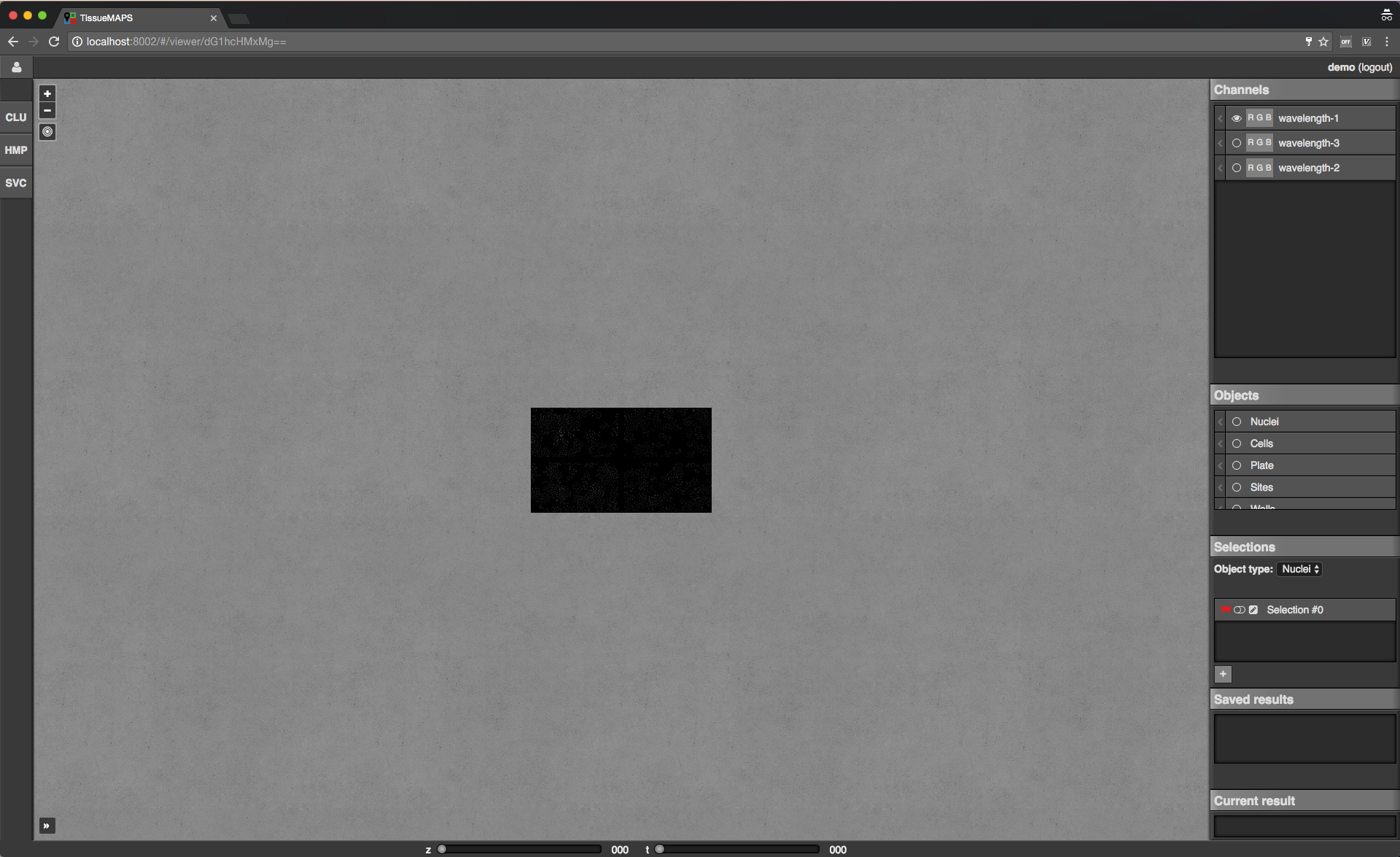
Viewer overview.
Upon initial access, the first channel is shown in the viewport at the maximally zoomed-out resultion level. You can zoom in and out using either the mouse wheel or trackpad or the + and - buttons provided at the top left corner of the viewport. The map can also be repositions within the viewport by dragging it with the mouse.
To the right of the viewport is the map sidebar and to the left the tool sidebar. Sections of the map control sidebar can be resized using the mouse and individual items can be rearranged via drag and drop. Below the viewport are sliders to zoom along the z-axis or time series for experiment comprised of images acquired at different z resolutions or time points, respectively.
The map sidebar has the following sections:
Channels: one raster image layer for each channel (created during the “pyramid_creation” workflow stage)Objects: one vector layer for each object type (created during the “image_analysis” workflow stage)Selections: tool for selecting mapobjects on the mapSaved results: one vector layer for each saved (previously generated) tool resultCurrent result: single vector layer for the most recent tool result
Individual sections are described in more detail below.
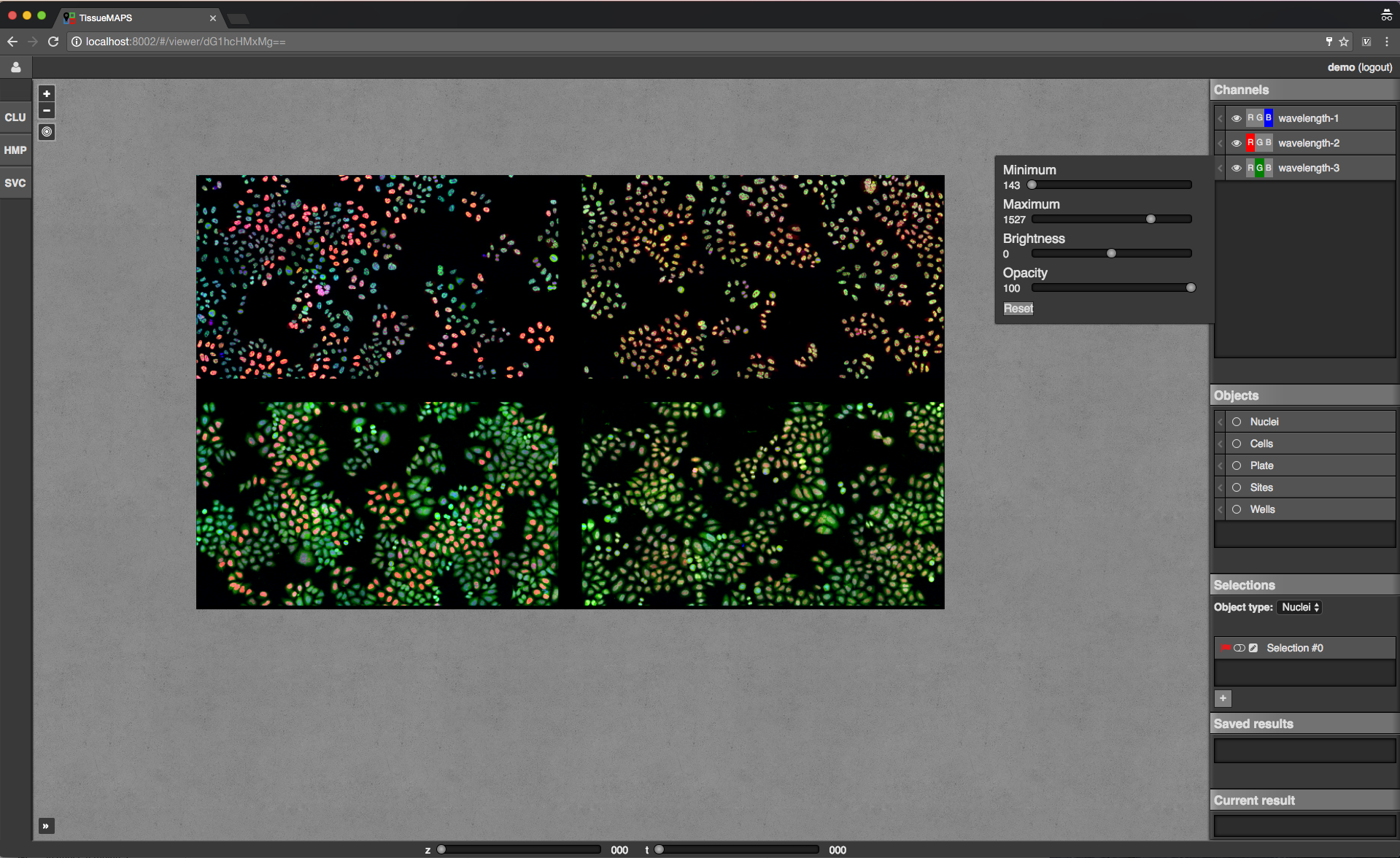
Map sidebar: Channels.
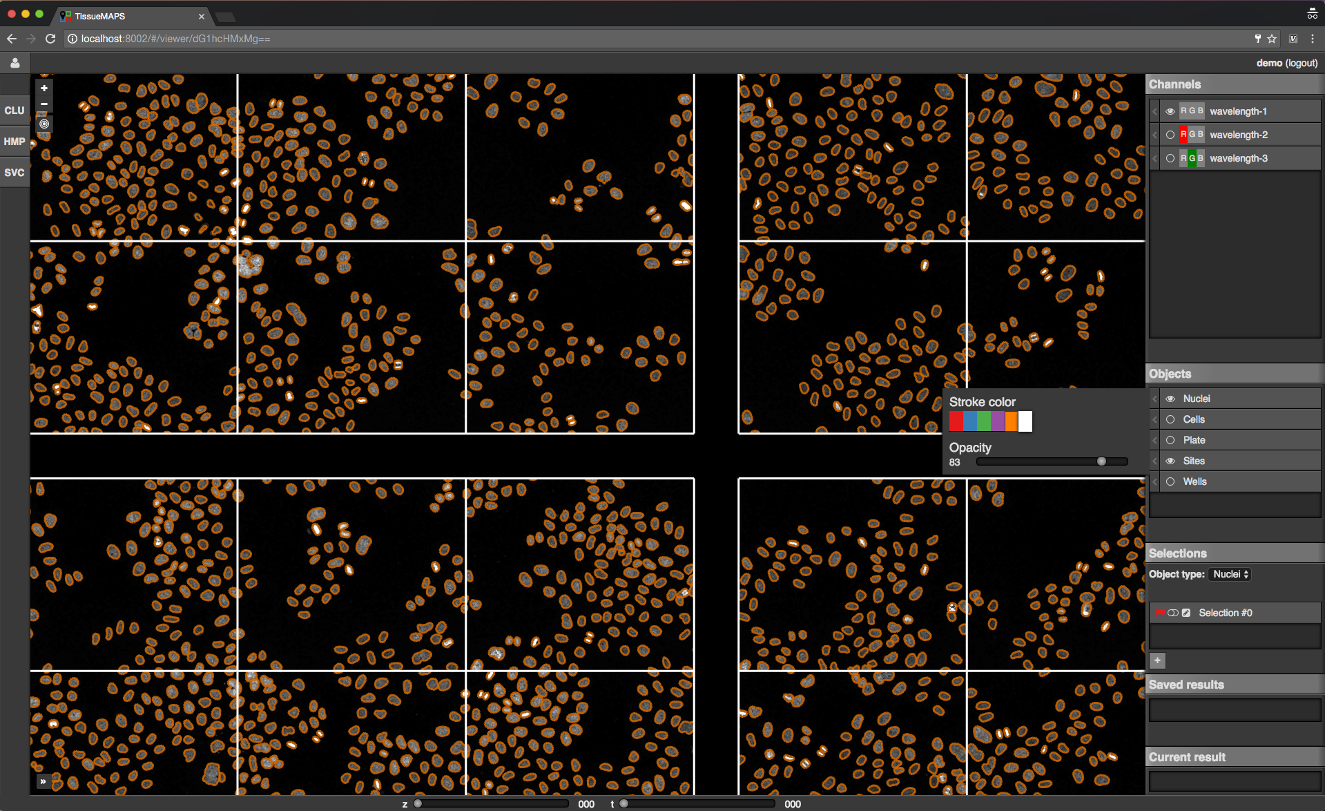
Map sidebar: Objects.
Note
Objects of type “Plates”, “Wells” and “Sites” will be auto-generated based on available image metadata. These static types are independent of parameters set in the “image_analysis” workflow stage.
Warning
Object outlines may not be represented 100% accurately on the map, because the polygon contours might have been simplified server side.
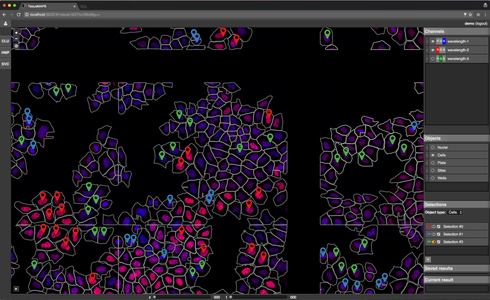
Map sidebar: Selections.
Data analysis tools
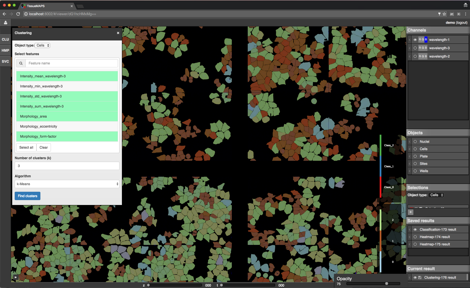
TissueMAPS provides a plugin framework for interactive data analysis tools. Available tools are listed in the tool sidebar to the left of the viewport.
Tool sidebar.
Each tool is associated with a separate window, which opens when the corresponding tool icon is clicked in the tool sidebar.
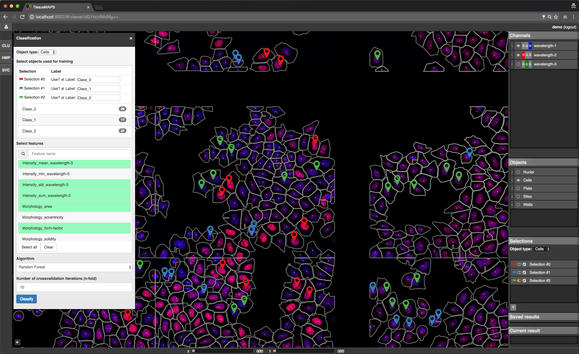
The window content varies between tools depending on their functionality. Typically, there is a section for selection of object types and features and a button to submit the tool request to the server. In case of the supervised classification (SVC) tool, there is also a section for assigning selections to label classes, which can be used for training of the classifier.
Let’s say you want to perform a supervised classification using the “SVC” tool based on labels provided in form of map selections (see above).
To perform the classification, select an object type (e.g. Cells) and one or more features from and click on  . This will submit a request to the server to perform the computation. Once the classification is done the result will appear in the “Current result” section of the map control sidebar.
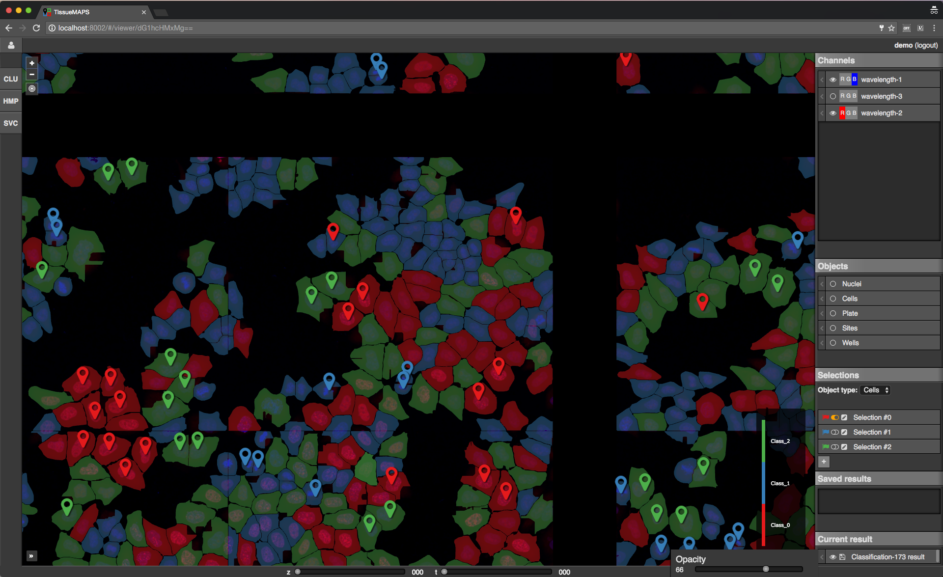
Map sidebar: Current result.
Map sidebar: Saved results.
RESTful programming
Clients use the REST API to access server side resources. In case of the user interface this is handled by the browser, but the same can be achieved in more programmatic, browser-independent way.
A request is composed of a resource specification provided in form of a Uniform Resource Locator (*URL*) and one of the following verbs: GET, PUT, POST or DELETE.
The server listens to routes that catch request messages, handles them and returns a defined response message to the client. This response includes a status code (e.g. 200) and the actual content. In addition, requests and responses have headers that hold information about their content, such as the media type (e.g. application/json or image/png).
Consider the following example: Let’s say you want to GET a list of your experiments. To this end, you can send the following request to the TissueMAPS server:
GET /api/experiments
The server would handle this response via the get_experiments() view function and respond with this message (using the example given in the user interface section):
HTTP/1.1 200 OK
Content-Type: application/json

{
    "data": [
        {
            "id": "MQ==",
            "name": "test",
            "description": "A very nice experiment that will get me into Nature",
            "user": "demo"
        }
    ]
}
The response has status code 200, meaning there were no errors, and the content of type application/json with the list of existing experiments. In this case, there is only one experiment named test that belongs to the demo user.
The same logic also applies to more complex query strings with additional parameters.
To download an image for a specific channel you could send a request like this:
GET /experiments/MQ==/channels/dG1hcHM0/image-file?plate_name=plate01,cycle_index=0,well_name=D03,x=0,y=0,tpoint=0,zplane=0
The server would respond with a message that contains the requested image as PNG-compressed binary data, which can be written to a file client-side using the provided filename:
HTTP/1.1 200 OK
Content-Type: image/png
Content-Disposition: attachment; filename="test_D03_x000_y000_z000_t000_wavelength-1.png"

...
Similarly, you can download all feature values extracted for a particular type of objects:
GET /api/experiments/MQ==/mapobjects/dG1hcHMx/feature-values
In this case, the server would respond with a message containing the requested feature values as CSV-encoded binary data, which can be written to a file using the provided filename:
HTTP/1.1 200 OK
Content-Type: application/octet-stream
Content-Disposition: attachment; filename="test_Cells_feature-values.csv"

...
For more information about available resources and verbs, please refer to tmserver.api.
Implementation
In principle, GET requests could be handled via the browser. You can try it by entering a URL into the browser address bar, e.g.:
http://localhost:8002/api/experiments
The server will responds with an error message with status code 401 (not authorized) because no access token was provided along with the request, which is required for JWT authentication.
So to make requests in practice, we need a client interface that is able to handle authentication. This can be achieved via the command line using cURL or through any other HTTP interface. In the following, we will demonstrate how requests can be handled in Python and Matlab:
Python example
import os
import requests
import json
import cv2
from StringIO import StringIO
import pandas as pd


def authenticate(url, username, password):
    response = requests.post(
        url + '/auth',
        data=json.dumps({'username': username, 'password': password}),
        headers={'content-type': 'application/json'}
    )
    response.raise_for_status()
    data = response.json()
    return data['access_token']


def http_get(url, api_uri, token, **params):
    response = requests.get(
        url + '/' + api_uri, params=params,
        headers={'Authorization': 'JWT ' + token}
    )
    response.raise_for_status()
    return response


def get_data(url, api_uri, token, **params):
    response = http_get(url, api_uri, token, params)
    data = response.json()
    return data['data']


def get_image(url, api_uri, token, **params):
    response = http_get(url, api_uri, token, params)
    data = response.content
    return cv2.imdecode(data)


def get_feature_values(url, api_uri, token, location, **params):
    response = http_get(url, api_uri, token, params)
    data = StringIO(response.content)
    return pd.from_csv(data)


if __name__ = '__main__':

    url = 'http://localhost:8002'

    # Login
    token = authenticate(url, 'demo', 'XXX')

    # GET list of existing experiments
    experiments = get_data(url, '/api/experiments', token)

    # GET image for a specific channel
    image = get_image(
        url, '/api/experiments/MQ==/channels/dG1hcHM0/image-files?
        plate_name=plate01,cycle_index=0,well_name=D03,well_pos_x=0,well_pos_y=0,
        tpoint=0,zplane=0',
        token
    )

    # GET feature values for a specific objects type
    data = get_feature_values(
        url, '/api/experiments/MQ==/mapobjects/dG1hcHMx/feature-values',
        token
    )
Matlab example
function [] = __main__()

    url = 'http://localhost:8002';

    % Login
    token = authenticate(url, 'demo', 'XXX');

    % GET list of existing experiments
    experiments = get_data(url, '/api/experiments', token);

    % GET image for a specific channel
    image = get_image(url, '/api/experiments/MQ==/channels/dG1hcHM0/image-files?plate_name=plate01,cycle_index=0,well_name=D03,well_pos_x=0,well_pos_y=0,tpoint=0,zplane=0', token);

    % GET feature values for a specific objects type
    data = get_feature_values(url, '/api/experiments/MQ==/mapobjects/dG1hcHMx/feature-values', token);

end


function token = authenticate(url, username, password)
    data = struct('username', username, 'password', password);
    options = weboptions('MediaType', 'application/json');
    response = webwrite([url, '/auth'], data, options);
    token = response.access_token;
end


function response = http_get(url, api_uri, token, varargin):
    options = weboptions('KeyName', 'Authorization', 'KeyValue', ['JWT ', token]);
    response = webread([url, '/', api_uri], options, varargin{:});
end


function data = get_data(url, api_uri, token, varargin)
    repsonse = http_get(url, api_uri, token, varargin);
    data = response.data;
end


function image = get_image(url, api_uri, token, varargin)
    image = http_get(url, api_uri, token, varargin);
end


function data = get_feature_values(url, api_uri, token, location, varagin)
    data = http_get(url, api_uri, token, varargin);
end
Python client
The tmclient package is a REST API wrapper that provides users the possibility to interact with the TissueMAPS server in a programmatic way. It abstracts the REST implementation and exposes objects and methods that don’t require any knowledge of RESTful programming.
Active programming interface
The TmClient class implements high-level methods for accessing resources without having to provide the actual resource indentifiers.
First, a TmClient object must be instantiated by providing the server address and login credentials:
from tmclient import TmClient

client = TmClient(
    host='localhost', port=8002, username='demo', password='XXX',
    experiment_name='test'
)
The instantiated object can then be used, for example, to download the pixels of a ChannelImageFile:
image = client.download_channel_image(
    channel_name='wavelength-1', plate_name='plate01', well_name='D03', well_pos_x=0, well_pos_y=0,
    cycle_index=0, tpoint=0, zplane=0, correct=True
)
The returned image object is an instance of NumPy ndarray:
# Show image dimensions
print image.shape

# Show first row of pixels
print image[0, :]
Similarly, FeatureValues for a particular MapobjectType can be downloaded as follows:
data = client.download_object_feature_values(mapobject_type='Cells')
In this case, the returned data object is an instance of Pandas DataFrame:
# Show names of features
print data.columns

# Iterate over objects
for index, values in data.iterrows():
    print index, values

# Iterate over features
for name, values in data.iteritems():
    print name, values
Command line interface
The tmclient Python package further provides the tm_client progam.
You can upload images and manage workflows entirely via the command line:
tm_client --help
Tip
You can store passwords in a ~/.tm_pass file as key-value pairs (username: password) in YAML format:
demo: XXX
This will allow you to omit the password argument in command line calls. This is not totally safe either, but at least your password won’t show up in the history and you don’t have to remember it.
The command line interface is structured according to the type of available resources, defined in tmserver.api.
To begin with, create the Experiment:
tm_client -vv -H localhost -P 8002 -u demo experiment create -n test
Note
You may want to override default values of parameters, such as microscope-type or workflow-type, depending on your use case.
Create a new Plate plate01:
tm_client -vv -H localhost -P 8002 -u demo plate -e test create --name plate01
Create a new Acquisition acquisition01 for plate plate01:
tm_client -vv -H localhost -P 8002 -u demo acquisition -e test create -p plate01 --name acquisition01
Upload each MicroscopeImageFile and MicroscopeMetadataFile for plate plate01 and acquisition acquisition01 from a local directory:
tm_client -vv -H localhost -P 8002 -u demo microscope-file -e test upload -p plate01 -a acquisition01 --directory ...
Check whether all files have been uploaded correctly:
tm_client -vv -H localhost -P 8002 -u demo microscope-file -e test ls -p plate01 -a acquisition01
To be able to process the uploaded images, you have to provide a WorkflowDescription. You can request a template and store it in a YAML file with either .yaml or .yml extension:
tm_client -vv -H localhost -P 8002 -u demo workflow -e test download --file /tmp/workflow.yml
Modify the workflow description acoording to your needs (as you would do in the workflow manager user interface) and upload it:
tm_client -vv -H localhost -P 8002 -u demo workflow -e test upload --file /tmp/workflow.yml
In case your workflow contains the jterator step, you will also have to provide a jterator project, i.e. a directory containing:
- a
PipelineDescriptionin form of apipeline.yamlYAML file- one
HandleDescriptionsin form of a*.handles.yamlYAML file for each module in the pipeline (in ahandlessubdirectory)
tm_client -vv -H localhost -P 8002 -u demo jtproject -e test upload --directory ...
Note
Handles file templates are available for each module in the JtModules repository. For additional information, please refer to tmlib.workflow.jterator.handles.
After workflow description and jtproject have been uploaded, you can submit the workflow for processing:
tm_client -vv -H localhost -P 8002 -u demo workflow -e test submit
You can subsequently monitor the workflow status:
tm_client -vv -H localhost -P 8002 -u demo workflow -e test status
Tip
You can use the program watch to periodically check the status:
watch -n 10 tm_client -H localhost -P 8002 -u demo workflow -e test status
Once the workflow is completed, you can download generated data:
Download the pixels content of a ChannelImageFile:
tm_client -vv -H localhost -P 8002 -u demo -p XXX channel-image -e test download -c wavelength-1 -p plate01 -w D03 -x 0 -y 0 -i 0 --correct
Download feature values for all objects of type Cells:
tm_client -vv -H localhost -P 8002 -u demo -p XXX feature-values -e test download -o Cells
Note
By default, files will be downloaded to your temporary directory, e.g. /tmp (the exact location depends on your operating system settings). The program will print the location of the file to the console when called with -vv or higher logging verbosity. You can specify an alternative download location for the download command using the --directory argument.
Using the library
The tmlibrary package implements an application programming interface (API) that represents an interface between the web application (implemented in the tmserver package) and storage and compute resources. The API provides routines for distributed computing and models for interacting with data stored on disk. The server uses the library and exposes part of its functionality to users via the RESTful API. Users with access to the server can also use the library directly. It further exposes command line interfaces (CLI), which provide users the possibility to interact with implemented programs via the console, which can be convenient for development, testing, and debugging.
Application programming interface (API)
Accessing data
Data can be accessed via model classes implemented in tmlib.models. Since data is stored (or referenced) in a database, a database connection must be established. This is achieved via the MainSession or ExperimentSession, depending on whether you need to access models derived from MainModel or ExperimentModel, respectively.
Model classes are implemented in form of SQLAlchemy Object Relational Mapper (ORM). For more information please refer to the ORM tuturial.
For example, a ChannelImage can be retrieved from a ChannelImageFile as follows (using the same parameters as in the examples above):
import tmlib.models as tm

with tm.utils.MainSession() as session:
    experiment = session.query(tm.ExperimentReference.id).\
        filter_by(name='test').\
        one()
    experiment_id = experiment.id

with tm.utils.ExperimentSession(experiment_id) as session:
    site = session.query(tm.Site.id).\
        join(tm.Well).\
        join(tm.Plate).\
        filter(
            tm.Plate.name == 'plate01',
            tm.Well.name == 'D03',
            tm.Site.x == 0,
            tm.Site.y == 0
        ).\
        one()
    image_file = session.query(tm.ChannelImageFile).\
        join(tm.Cycle).\
        join(tm.Channel).\
        filter(
            tm.Cycle.index == 0,
            tm.Channel.name == 'wavelength-1',
            tm.ChannelImageFile.site_id == site.id,
            tm.ChannelImageFile.tpoint == 0,
            tm.ChannelImageFile.zplane == 0
        ).\
        one()
    image = image_file.get()
Warning
Some experiment-specific database tables are distributed, i.e. small fractions (so called “shards”) are spread across different database servers for improved performance. Rows of these tables can still be selected via the ExperimentSession, but they can not be modified within a session (see ExperimentConnection). In addition, distributed tables do not support sub-queries and cannot be joined with standard, non-distributed tables.
Warning
Content of files should only be accessed via the provided get and put methods of the respective model class implemented in tmlib.models.file, since the particular storage backend (e.g. filesystem or object storage) may be subject to change.
Command line interface (CLI)
A Workflow and each individual WorkflowStep can also be controlled via the command line.
Managing workflow steps
Each WorkflowStep represents a separate program that exposes its own command line interface. These interfaces have are a very similar structure and provide sub-commands for methods defined in either the CommandLineInterface base class or the step-specific implementation.
The name of the step is also automatically the name of the command line program. For example, the jterator program can be controlled via the jterator command.
You can initialize the step via the init sub-command:
jterator -vv 1 init --batch_size 5
or shorthand:
jterator -vv 1 init -b 5
And then run jobs:
either individually on the local machine via the
runsub-command:jterator -vv 1 run -j 1
or submit them for parallel processing on remote machines via the
submitsub-command:jterator -vv 1 submit
Note
The submit command internally calls the program with run --job <job_id> on different CPUs of the same machine or on other remote machines for each of the batch jobs defined via init.
To print the description of an individual job to the console call the info sub-command:
jterator -vv 1 info --phase run --job 1
You can further print the standard output or error of a job via the log sub-command:
jterator -vv 1 log --phase run --job 1
Note
The detail of log messages depends on the logging level, which is specified via the --verbosity or -v argument. The more vs the more detailed the log output becomes.
The full documentation of each command line interface is available online along with the documentation of the respective cli module, e.g. tmlib.workflow.jterator.cli, or via the console by calling the program with --help or -h:
jterator -h
Managing workflows
Distributed image processing workflows can be set up and submitted via the workflow manager user interface. The same can be achieved via the command line through the tm_workflow program.
Submitting the workflow for experiment with ID 1 is as simple as:
tm_workflow -vv 1 submit
The workflow can also be resubmitted at a given stage:
tm_workflow -vv 1 resubmit --stage image_preprocessing
Note
Names of workflow stages may contain underscores. They are stripped for display in the user interface, but are required in the command line interface.
